第十章
内容
第十章
零、练一练
练一练
请尝试在pd.Timestamp()中传入其他格式的时刻字符串,如:“20210901”、“2021-09-01”等,体会该构造方法的灵活性。
pd.Timestamp("20210901")
Timestamp('2021-09-01 00:00:00')
pd.Timestamp("2021-09-01")
Timestamp('2021-09-01 00:00:00')
练一练
请分别将如下格式的时间戳列表转为正确的时序Series格式。
["0901 2021", "0902 2021", "0903 2021"]
["21-9-1 8-35-50", "21-9-2 9-25-45"]
1
bad_format = ["0901 2021", "0902 2021", "0903 2021"]
temp = pd.to_datetime(bad_format, format='%m%d %Y')
temp
DatetimeIndex(['2021-09-01', '2021-09-02', '2021-09-03'], dtype='datetime64[ns]', freq=None)
bad_format = ["2021-9-1 8-35-50", "2021-9-2 9-25-45"]
temp = pd.to_datetime(bad_format, format='%Y-%m-%d %H-%M-%S')
temp
DatetimeIndex(['2021-09-01 08:35:50', '2021-09-02 09:25:45'], dtype='datetime64[ns]', freq=None)
练一练
Timestamp对象上定义了1个value属性,其返回的整数值代表了从1970年1月1日零点到给定时间戳相差的纳秒数。同时,pd.Timestamp也支持通过这个整数值来构造时间戳,即它们之间一一对应。请利用这个特性设计1个随机生成给定日期区间内日期序列的函数random_dates(time1, time2, n),其中time1、time2和n分别指区间左边界、区间右边界和序列元素个数。
def random_dates(time1, time2, n):
    t1 = pd.Timestamp(time1).value / 1e9
    t2 = pd.Timestamp(time2).value / 1e9
    d = np.random.randint(t1, t2+1, n)
    return pd.to_datetime(d * 1e9)
random_dates("20200101", "20200105", 4)
DatetimeIndex(['2020-01-04 12:55:11', '2020-01-02 08:45:52',
               '2020-01-02 18:18:35', '2020-01-04 12:28:57'],
              dtype='datetime64[ns]', freq=None)
练一练
在上述构造的Series中,按如下要求选出子序列:
选出每月前十天中的工作日
选出每月的1号、11号和21号以及每月的最后5天
s = pd.Series(
    np.random.randint(2,size=365),
    index=pd.date_range('2021-01-01','2021-12-31'))
idx = pd.Series(s.index).dt
s.head()
2021-01-01    1
2021-01-02    1
2021-01-03    0
2021-01-04    0
2021-01-05    1
Freq: D, dtype: int32
1
res = s[(idx.day<=10).values]
res.head()
2021-01-01    1
2021-01-02    1
2021-01-03    0
2021-01-04    0
2021-01-05    1
dtype: int32
2
res = s[((idx.daysinmonth-idx.day<=4)|(idx.day%10==1)).values]
res.head()
2021-01-01    1
2021-01-11    1
2021-01-21    0
2021-01-27    1
2021-01-28    0
dtype: int32
练一练
与时间戳序列类似,时间差序列也可以使用max()、min()和mean()来得到最大时间差、最小时间差以及平均时间差,请基于learn_pandas数据集中的Time_Record列(学生的跑步体侧成绩)解决如下问题:
最慢的学生花费的秒数是最快学生的几倍?
在跑步时间超过及格线4分30秒的学生中(即不及格的学生中),每10秒做一次划分(区间左闭右开),请计算每一个区间(4分30秒至4分40秒、4分40秒至4分50秒、...)的学生人数。
1
df = pd.read_csv("data/learn_pandas.csv")
df.Time_Record = pd.to_timedelta(df.Time_Record)
df.Time_Record.dt.seconds.max() / df.Time_Record.dt.seconds.min()
1.5592417061611374
2
s = df.Time_Record[df.Time_Record > pd.Timedelta("4m30s")].reset_index(drop=True)
pd.to_timedelta((s // pd.Timedelta("10s") * 10), unit="s").value_counts().sort_index()
0 days 00:04:30    15
0 days 00:04:40    12
0 days 00:04:50    16
0 days 00:05:00    18
0 days 00:05:10    20
0 days 00:05:20    24
Name: Time_Record, dtype: int64
练一练
将上述的pd.offsets.BDay(30)改为pd.offsets.BDay(12),请问2021-09-06和2021-09-05经过如上的操作后结果仍然保持不一致吗?请说明理由。
由于两个日期过了12个工作日之后,都是九月二十二日,因此它们的结果一致:
pd.Timestamp('20210906') + pd.offsets.BDay(12) - pd.Timestamp('20210906')
Timedelta('16 days 00:00:00')
pd.Timestamp('20210905') + pd.offsets.BDay(12) - pd.Timestamp('20210905')
Timedelta('16 days 00:00:00')
练一练
请利用10.1.4节介绍的索引方法,构造与上述bdate_range()结果一致的DatetimeIndex。(练习重点在于使用dt对象和布尔序列的组合,来模拟weekmask和holidays的筛选过程)
s = pd.Series(pd.date_range(start='20210920', end='20211015'))
s = s[((s>pd.Timestamp("20211007"))|(s<pd.Timestamp("20211001"))).values]
s = s[s.dt.dayofweek.between(2,5).values].values
s = pd.to_datetime(s)
s
DatetimeIndex(['2021-09-22', '2021-09-23', '2021-09-24', '2021-09-25',
               '2021-09-29', '2021-09-30', '2021-10-08', '2021-10-09',
               '2021-10-13', '2021-10-14', '2021-10-15'],
              dtype='datetime64[ns]', freq=None)
练一练
在日期偏置中我们介绍了CDay,它能够对节假日和部分星期进行筛选。假设现在需要对所有周二以及每月的第一个周末进行过滤,从而进行7个Custom Day的滑窗操作,请仿照上面的例子给出解决方案。
s = pd.Series(np.random.randint(0, 10, 365),
              index=pd.date_range("20210101","20211231"))
s = s.sample(250, random_state=999).sort_index()
idx = pd.Series(s.index).dt
s_cday = s[((idx.dayofweek!=1)&((idx.day>7)|((idx.day<7)&(idx.day_of_week<5)))).values]
cday_sum = s_cday.rolling(7, min_periods=1).sum()
result = cday_sum.reindex(s.index).ffill()
result.head(8)
2021-01-01     1.0
2021-01-02     1.0
2021-01-04     2.0
2021-01-05     2.0
2021-01-07     2.0
2021-01-08     7.0
2021-01-09    12.0
2021-01-11    17.0
dtype: float64
练一练
对上述数据每天按照0点至12点、12点至24点进行分组极差计算。
np.random.seed(0)
idx = pd.date_range("20210901", "20210902 23:59:59", freq="90min")
s = pd.Series(np.random.rand(idx.shape[0]), index=idx)
s.resample("12H").apply(lambda x: x.max()-x.min())
2021-09-01 00:00:00    0.468118
2021-09-01 12:00:00    0.892627
2021-09-02 00:00:00    0.958400
2021-09-02 12:00:00    0.826394
Freq: 12H, dtype: float64
练一练
对于merge_asof()而言,只需要保证键是有序且可比较的即可,因此整数和浮点的模糊匹配也是可以进行的。请举出1个非时序的例子来说明参数选择对合并结果的影响。
df1 = pd.DataFrame({
    "A": [2,4,6,8,10],
})
df1
| A | |
|---|---|
| 0 | 2 |
| 1 | 4 |
| 2 | 6 |
| 3 | 8 |
| 4 | 10 |
df2 = pd.DataFrame({
    "A": [1,3,5,6,9],
    "B": range(100,105)
})
df2
| A | B | |
|---|---|---|
| 0 | 1 | 100 |
| 1 | 3 | 101 |
| 2 | 5 | 102 |
| 3 | 6 | 103 |
| 4 | 9 | 104 |
pd.merge_asof(df1, df2, on="A", direction="backward")
| A | B | |
|---|---|---|
| 0 | 2 | 100 |
| 1 | 4 | 101 |
| 2 | 6 | 103 |
| 3 | 8 | 103 |
| 4 | 10 | 104 |
一、太阳辐射数据的时序分析
现有1份关于太阳辐射的数据集:
df = pd.read_csv('data/ch10/solar.csv',
                 usecols=['Data','Time','Radiation','Temperature'])
df.head(2)
| Data | Time | Radiation | Temperature | |
|---|---|---|---|---|
| 0 | 9/29/2016 12:00:00 AM | 23:55:26 | 1.21 | 48 |
| 1 | 9/29/2016 12:00:00 AM | 23:50:23 | 1.21 | 48 |
将Datetime列和Time列合并为1个时间列Datetime,同时把它作为索引后排序。
每条记录时间的间隔显然并不一致,请解决如下问题:
找出间隔时间的前3个最大值所对应的3组时间戳。
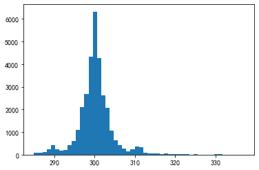
是否存在1个大致的范围,使得绝大多数的间隔时间都落在这个区间中?如果存在,请对此范围内的样本间隔秒数画出直方图,设置bins=50。(直方图的画法可见11.1.1节)
求如下指标对应的Series:
温度与辐射量的6小时滑动相关系数
以三点、九点、十五点、二十一点为分割,该观测所在时间区间的温度均值序列
每条观测记录6小时前的辐射量(一般而言不会恰好取到,此时取最近时间戳对应的辐射量)
【解答】
1
df = pd.read_csv('data/ch10/solar.csv', usecols=['Data','Time',
                 'Radiation','Temperature'])
solar_date = df.Data.str.extract('([/|\w]+\s).+')[0]
df['Data'] = pd.to_datetime(solar_date + df.Time)
df = df.drop(columns='Time').rename(columns={'Data':'Datetime'}
            ).set_index('Datetime').sort_index()
df.head(3)
| Radiation | Temperature | |
|---|---|---|
| Datetime | ||
| 2016-09-01 00:00:08 | 2.58 | 51 |
| 2016-09-01 00:05:10 | 2.83 | 51 |
| 2016-09-01 00:20:06 | 2.16 | 51 |
2-1
s = df.index.to_series().reset_index(drop=True).diff().dt.total_seconds()
max_3 = s.nlargest(3).index
df.index[max_3.union(max_3-1)]
DatetimeIndex(['2016-09-29 23:55:26', '2016-10-01 00:00:19',
               '2016-11-29 19:05:02', '2016-12-01 00:00:02',
               '2016-12-05 20:45:53', '2016-12-08 11:10:42'],
              dtype='datetime64[ns]', name='Datetime', freq=None)
res = s.mask((s>s.quantile(0.99))|(s<s.quantile(0.01)))
_ = plt.hist(res, bins=50)
3-1
res = df.Radiation.rolling('6H').corr(df.Temperature)
res.tail(3)
Datetime
2016-12-31 23:45:04    0.328574
2016-12-31 23:50:03    0.261883
2016-12-31 23:55:01    0.262406
dtype: float64
3-2
res = df.Temperature.resample('6H', origin='03:00:00').mean()
res.head(3)
Datetime
2016-08-31 21:00:00    51.218750
2016-09-01 03:00:00    50.033333
2016-09-01 09:00:00    59.379310
Freq: 6H, Name: Temperature, dtype: float64
3-3
temp = pd.Series(df.index.shift(freq='-6H'), name="Datetime").to_frame()
res = pd.merge_asof(temp, df.Radiation.to_frame().reset_index(), on="Datetime", direction="nearest")
res.tail()
| Datetime | Radiation | |
|---|---|---|
| 32681 | 2016-12-31 17:35:02 | 15.96 |
| 32682 | 2016-12-31 17:40:01 | 11.98 |
| 32683 | 2016-12-31 17:45:04 | 9.33 |
| 32684 | 2016-12-31 17:50:03 | 8.49 |
| 32685 | 2016-12-31 17:55:01 | 5.84 |
二、水果销量分析
现有1份2019年每日水果销量记录表:
df = pd.read_csv('data/ch10/fruit.csv')
df.head(2)
| Date | Fruit | Sale | |
|---|---|---|---|
| 0 | 2019-04-18 | Peach | 15 |
| 1 | 2019-12-29 | Peach | 15 |
统计如下指标:
每月上半月(15号及之前)与下半月葡萄销量的比值
每月最后一天的生梨销量总和
每月最后一天工作日的生梨销量总和
每月最后五天的苹果销量均值
按月计算周一至周日各品种水果的平均记录条数(例如苹果在1月的4个周一记录条数分别为13、10、12和11,则其平均记录条数为11.5),行索引外层为水果名称,内层为月份,列索引为星期。
按天计算向前10个工作日窗口的苹果销量均值序列,非工作日的值用上一个工作日的结果填充。
【解答】
1-1
df = pd.read_csv('data/ch10/fruit.csv')
df.Date = pd.to_datetime(df.Date)
df_grape = df.query("Fruit == 'Grape'")
res = df_grape.groupby([np.where(df_grape.Date.dt.day<=15,
                        'First', 'Second'),df_grape.Date.dt.month]
                        )['Sale'].mean().to_frame().unstack(0
                        ).droplevel(0,axis=1)
res = (res.First/res.Second).rename_axis('Month')
res.head()
Month
1    1.174998
2    0.968890
3    0.951351
4    1.020797
5    0.931061
dtype: float64
1-2
df[df.Date.dt.is_month_end].query("Fruit == 'Pear'").groupby('Date').Sale.sum().head()
Date
2019-01-31    847
2019-02-28    774
2019-03-31    761
2019-04-30    648
2019-05-31    616
Name: Sale, dtype: int64
1-3
df[df.Date.isin(pd.date_range('20190101', '20191231',
                    freq='BM'))].query("Fruit == 'Pear'"
                    ).groupby('Date').Sale.mean().head()
Date
2019-01-31    60.500000
2019-02-28    59.538462
2019-03-29    56.666667
2019-04-30    64.800000
2019-05-31    61.600000
Name: Sale, dtype: float64
1-4
target_dt = df.drop_duplicates().groupby(df.Date.drop_duplicates(
            ).dt.month)['Date'].nlargest(5).reset_index(drop=True)
res = df.set_index('Date').loc[target_dt].reset_index(
            ).query("Fruit == 'Apple'")
res = res.groupby(res.Date.dt.month)['Sale'].mean(
            ).rename_axis('Month')
res.head()
Month
1    65.313725
2    54.061538
3    59.325581
4    65.795455
5    57.465116
Name: Sale, dtype: float64
2
month_order = ['January','February','March','April',
                'May','June','July','August','September',
                'October','November','December']
week_order = ['Mon','Tue','Wed','Thu','Fri','Sat','Sum']
group1 = df.Date.dt.month_name().astype('category').cat.reorder_categories(
        month_order, ordered=True)
group2 = df.Fruit
group3 = df.Date.dt.dayofweek.replace(dict(zip(range(7),week_order))
         ).astype('category').cat.reorder_categories(
         week_order, ordered=True)
res = df.groupby([group1, group2,group3])['Sale'].count().to_frame(
         ).unstack(0).droplevel(0,axis=1)
res.head()
| Date | January | February | March | April | May | June | July | August | September | October | November | December | |
|---|---|---|---|---|---|---|---|---|---|---|---|---|---|
| Fruit | Date | ||||||||||||
| Apple | Mon | 46 | 43 | 43 | 47 | 43 | 40 | 41 | 38 | 59 | 42 | 39 | 45 |
| Tue | 50 | 40 | 44 | 52 | 46 | 39 | 50 | 42 | 40 | 57 | 47 | 47 | |
| Wed | 50 | 47 | 37 | 43 | 39 | 39 | 58 | 43 | 35 | 46 | 47 | 38 | |
| Thu | 45 | 35 | 31 | 47 | 58 | 33 | 52 | 44 | 36 | 63 | 37 | 40 | |
| Fri | 32 | 33 | 52 | 31 | 46 | 38 | 37 | 48 | 34 | 37 | 46 | 41 |
3
df_apple = df[(df.Fruit=='Apple')&(
              ~df.Date.dt.dayofweek.isin([5,6]))]
s = pd.Series(df_apple.Sale.values,
              index=df_apple.Date).groupby('Date').sum()
res = s.rolling('10D').mean().reindex(
              pd.date_range('20190101','20191231')).fillna(method='ffill')
res.head()
2019-01-01    189.000000
2019-01-02    335.500000
2019-01-03    520.333333
2019-01-04    527.750000
2019-01-05    527.750000
Freq: D, dtype: float64
三、使用Prophet进行时序预测
Prophet是一个用于时序数据预测的工具包,它对于周期性或趋势性的时序数据具有良好的拟合预测能力,通过如下pip命令可进行安装:
$ conda install -c conda-forge prophet
Prophet模型假设目标变量\(y(t)\)可以被分解为三个部分:
其中,\(g(t)\)为趋势函数,\(s(t)\)为周期函数,\(h(t)\)为节假日效应函数,\(\epsilon\)为随机误差。Prophet默认使用分段线性函数(自动检测分段点)来表示\(g(t)\)的部分,使用有限项傅里叶级数来表示\(s(t)\)部分。\(h(t)\)有关节假日相关的操作请读者自行在官方文档查询相关操作。
在data/ch10/prophet_ts1.csv中存放了一条时间序列的相关特征,使用matplotlib(第十一章详细介绍)进行可视化后可以发现图10.5的趋势可被分为三段,每段都以年为周期变化:
import matplotlib.pyplot as plt

df = pd.read_csv("data/ch10/prophet_ts1.csv", parse_dates=["ds"])
plt.scatter(df.ds, df.y, s=0.1)

图10.5 prophet_ts1数据的时序趋势
此时,可以用Prophet进行以年(365天)为周期的模型拟合:
from prophet import Prophet

# 关闭所有预设的周期
model = Prophet(
    weekly_seasonality=False,
    yearly_seasonality=False,
    daily_seasonality=False,
    # 模型可以自动检测分段点,也可以手动添加
    # changepoints=['2003-07-29', "2010-02-22"],
)
# 人工添加365天的年周期,fourier_order表示傅里叶级数的阶数,参数可调节
# 此外,可以添加多种周期性,例如先添加365的年周期,再添加7的周周期
# 此时s(t) = s_{year}(t) + s_{week}(t)
model.add_seasonality(name='year_change', period=365, fourier_order=3)
model.fit(df)
Importing plotly failed. Interactive plots will not work.
C:\Users\gyh\miniconda3\envs\final\lib\site-packages\prophet\forecaster.py:896: FutureWarning: The frame.append method is deprecated and will be removed from pandas in a future version. Use pandas.concat instead.
  components = components.append(new_comp)
<prophet.forecaster.Prophet at 0x1fec05dedf0>
接着,使用模型对后续四年的情况进行预测:
future = model.make_future_dataframe(periods=365*4)
res = model.predict(future)[['ds', 'yhat']]
C:\Users\gyh\miniconda3\envs\final\lib\site-packages\prophet\forecaster.py:896: FutureWarning: The frame.append method is deprecated and will be removed from pandas in a future version. Use pandas.concat instead.
  components = components.append(new_comp)
C:\Users\gyh\miniconda3\envs\final\lib\site-packages\prophet\forecaster.py:896: FutureWarning: The frame.append method is deprecated and will be removed from pandas in a future version. Use pandas.concat instead.
  components = components.append(new_comp)
用红色表示对过去的拟合曲线,用蓝色表示对未来的预测曲线进行绘制,结果如图10.6所示:
plt.scatter(df.ds, df.y, s=0.1)
plt.plot(res.ds[:df.shape[0]], res.yhat[:df.shape[0]], c="Red")
plt.plot(res.ds[df.shape[0]:], res.yhat[df.shape[0]:], c="Blue")

图10.6 prophet_ts1数据的拟合和预测结果
但有些时候数据特征的周期振幅会随着时间变化,例如在data/ch10/prophet_ts2.csv中,越靠后的年份波动性越强,可视化情况如图10.7所示。
df = pd.read_csv("data/ch10/prophet_ts2.csv", parse_dates=["ds"])
plt.scatter(df.ds, df.y, s=0.1)

图10.7 prophet_ts2数据的时序趋势
默认情况下Prophet使用加法模型,即seasonality_mode参数为“additive”,此时可以将其更改为“multiplicative”,表示乘法模型,即
此时,仿照上述过程进行拟合,对结果仍然用蓝色和红色区分未来预测和历史拟合,可视化效果如图10.8所示:
model = Prophet(
    weekly_seasonality=False,
    yearly_seasonality=False,
    daily_seasonality=False,
    seasonality_mode="multiplicative"
)
model.add_seasonality(name='year_change', period=365, fourier_order=3)
model.fit(df)
future = model.make_future_dataframe(periods=365*4)
res = model.predict(future)[['ds', 'yhat']]
plt.scatter(df.ds, df.y, s=0.1)
plt.plot(res.ds[:df.shape[0]], res.yhat[:df.shape[0]], c="Red")
plt.plot(res.ds[df.shape[0]:], res.yhat[df.shape[0]:], c="Blue")

图10.8 prophet_ts2数据的拟合和预测结果
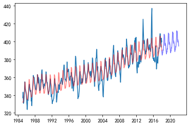
在data/ch10/prophet_data.csv中存放了8组从1985年1月至2017年12月的时序特征,完成以下任务:
以1985年1月至2014年12月为训练集,以2015年1月至2017年12月为验证集,以均方误差(MSE)为评价指标,分别对8组特征选择对应的模型最优参数,可调节的参数包括但不限于分割点changepoints、模型形式seasonality_mode以及通过add_seasonality添加的潜在周期模式。
分别对8组时序特征进行预测,预测范围为2018年1月至2021年12月。
【解答】
此处仅演示Sequence_1+调节fourier_order参数,其余类似:
1
df = pd.read_csv("data/ch10/prophet_data.csv")
df_seq = df.iloc[:, [0]].copy().rename(columns={"Sequence_1":"y"})
df_seq["ds"] = pd.date_range("19850101", "20171231", freq="M")
df_seq = df_seq[["ds", "y"]]
def get_order():
    min_mse = float("inf")
    order_list = [3,5,8]
    final_order = None
    for order in order_list:
        model = Prophet(
            weekly_seasonality=False,
            yearly_seasonality=False,
            daily_seasonality=False,
        )
        model.add_seasonality(
            name='year_change', period=365, fourier_order=order)
        model.fit(df_seq.iloc[:-36])
        predict = model.predict(df_seq.ds.iloc[-36:].to_frame()).yhat
        mse = ((df_seq.y.iloc[-36:].reset_index(drop=True) - predict) ** 2).mean()
        if mse < min_mse:
            final_order = order
            min_mse = mse
    return final_order
model = Prophet(
    weekly_seasonality=False,
    yearly_seasonality=False,
    daily_seasonality=False,
)
model.add_seasonality(name='year_change', period=365, fourier_order=get_order())
model.fit(df_seq)
C:\Users\gyh\miniconda3\envs\final\lib\site-packages\prophet\forecaster.py:896: FutureWarning: The frame.append method is deprecated and will be removed from pandas in a future version. Use pandas.concat instead.
  components = components.append(new_comp)
C:\Users\gyh\miniconda3\envs\final\lib\site-packages\prophet\forecaster.py:896: FutureWarning: The frame.append method is deprecated and will be removed from pandas in a future version. Use pandas.concat instead.
  components = components.append(new_comp)
C:\Users\gyh\miniconda3\envs\final\lib\site-packages\prophet\forecaster.py:896: FutureWarning: The frame.append method is deprecated and will be removed from pandas in a future version. Use pandas.concat instead.
  components = components.append(new_comp)
C:\Users\gyh\miniconda3\envs\final\lib\site-packages\prophet\forecaster.py:896: FutureWarning: The frame.append method is deprecated and will be removed from pandas in a future version. Use pandas.concat instead.
  components = components.append(new_comp)
C:\Users\gyh\miniconda3\envs\final\lib\site-packages\prophet\forecaster.py:896: FutureWarning: The frame.append method is deprecated and will be removed from pandas in a future version. Use pandas.concat instead.
  components = components.append(new_comp)
C:\Users\gyh\miniconda3\envs\final\lib\site-packages\prophet\forecaster.py:896: FutureWarning: The frame.append method is deprecated and will be removed from pandas in a future version. Use pandas.concat instead.
  components = components.append(new_comp)
C:\Users\gyh\miniconda3\envs\final\lib\site-packages\prophet\forecaster.py:896: FutureWarning: The frame.append method is deprecated and will be removed from pandas in a future version. Use pandas.concat instead.
  components = components.append(new_comp)
C:\Users\gyh\miniconda3\envs\final\lib\site-packages\prophet\forecaster.py:896: FutureWarning: The frame.append method is deprecated and will be removed from pandas in a future version. Use pandas.concat instead.
  components = components.append(new_comp)
C:\Users\gyh\miniconda3\envs\final\lib\site-packages\prophet\forecaster.py:896: FutureWarning: The frame.append method is deprecated and will be removed from pandas in a future version. Use pandas.concat instead.
  components = components.append(new_comp)
C:\Users\gyh\miniconda3\envs\final\lib\site-packages\prophet\forecaster.py:896: FutureWarning: The frame.append method is deprecated and will be removed from pandas in a future version. Use pandas.concat instead.
  components = components.append(new_comp)
<prophet.forecaster.Prophet at 0x1feccd8bb20>
2
future = model.make_future_dataframe(periods=365*4)
res = model.predict(future)[['ds', 'yhat']]
plt.plot(df_seq.ds, df.iloc[:,0])
plt.plot(res.ds[:df.shape[0]], res.yhat[:df.shape[0]], c="Red", alpha=0.5)
plt.plot(res.ds[df.shape[0]:], res.yhat[df.shape[0]:], c="Blue", alpha=0.5)
C:\Users\gyh\miniconda3\envs\final\lib\site-packages\prophet\forecaster.py:896: FutureWarning: The frame.append method is deprecated and will be removed from pandas in a future version. Use pandas.concat instead.
  components = components.append(new_comp)
C:\Users\gyh\miniconda3\envs\final\lib\site-packages\prophet\forecaster.py:896: FutureWarning: The frame.append method is deprecated and will be removed from pandas in a future version. Use pandas.concat instead.
  components = components.append(new_comp)
[<matplotlib.lines.Line2D at 0x1fed21cb460>]