第十一章
内容
第十一章
零、练一练
练一练
事实上,hist函数是有返回值的,只不过在大多数情况下用户并不关心。Python中,常把不需要的返回值赋给“_”变量,此处也正是这样做的。请观察hist的返回值,并尝试说明其含义。
data = np.random.randn(100)
val = plt.hist(data)
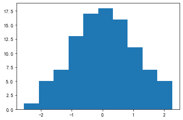
第一个返回值是hist分箱结果中每个箱子的样本数量:
val[0]
array([ 1., 5., 7., 13., 17., 18., 16., 11., 7., 5.])
第二个返回值是分箱的边界值,n个箱子会产生n+1个边界:
val[1]
array([-2.55298982, -2.07071537, -1.58844093, -1.10616648, -0.62389204,
       -0.1416176 ,  0.34065685,  0.82293129,  1.30520574,  1.78748018,
        2.26975462])
第三个返回值是matplotlib中的patches对象
val[2]
<BarContainer object of 10 artists>
练一练
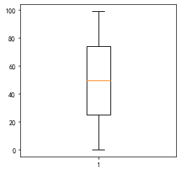
在上图中,数据值为2的新增样本点没有被判定为异常,请通过计算说明理由。
np.random.seed(0)
data = np.random.randn(100)
data = data.tolist() + [2,3,4] # 引入一些较大的值
_ = plt.boxplot(data)
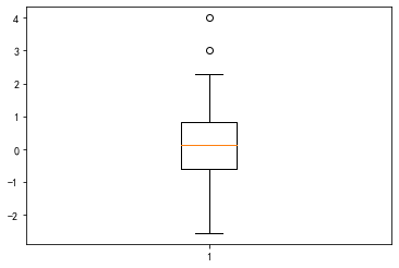
q75 = np.quantile(data, 0.75)
q25 = np.quantile(data, 0.25)
threshold  = q75 + 1.5*(q75 - q25)
data = np.array(data)
data[data <= threshold].max() # 高于2
2.2697546239876076
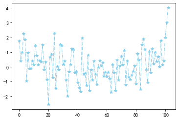
练一练
请尝试不同参数的组合,观察plt.plot()的绘图结果。
_ = plt.plot(data, linewidth=1.0, color="skyblue", marker="*", linestyle="-.")
练一练
请对比柱状图和直方图,总结它们之间的区别和联系。
直方图一般用于查看连续变量的离散化分布,柱状图一般用于查看离散化变量的频数或频率统计情况。
练一练
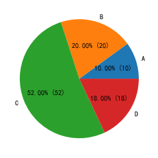
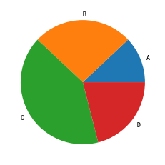
在pie函数中,可以将autopct参数设定为一个单个输入值的函数,其输入值含义是每个类别的占比乘以100,其输出值为字符串。若想在饼图的每一个部分添加占比的数字描述,可以令该参数为lambda p: "%.1f%%"%p,其中%.1f将p保留一位小数,%%表示百分号(%自身在Python格式化字符中需要通过两个%转义)。若现在想要把描述改为“占比 (个数)”的格式,例如当前类别占比5%,共计样本10个,保留2位小数,那么就应当显式为“5.00% (10)”,请利用autopct参数实现。
s = pd.Series(np.random.choice(list("ABCD"), size=100, p=[0.1,0.2,0.5,0.2]))
data = s.value_counts().sort_index()
_ = plt.pie(data.values, labels=data.index, autopct=lambda p: "%.2f%% (%d)"%(p,round(p*s.shape[0]/100)))
练一练
如果上述data是5维的,我们还能通过何种策略来体现第五个维度的数据取值?
使用scatter图不同的marker
使用有边框的圆和没有边框的圆
使用不同颜色的映射组(比如浅蓝到深蓝、浅红到深红)
使用子图绘制
练一练
在高维数据中,类别型数据和数值型数据的展示方式是不同的。请分别总结一些相应的展示策略,并构造相应的例子进行绘图。
答案因人而异,但需要指出的是,类别型和数据型展示策略的区别在于,前者在图像上的控制参数是离散化的(是否有边框、属于哪个子图、使用哪种marker),而后者在图像上的控制参数是连续的(连续数据本身的取值、marker的size、line的粗细、透明度)。
练一练
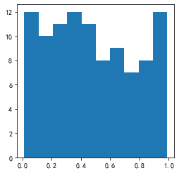
与plt.hist()类似,用户也能通过ax.hist()来进行绘图。先前介绍的基本绘图类型(boxplot、pie、bar等等)是否都能在ax对象上实现?请查阅matplotlib.axes模块对应的api文档,并给出例子说明。
可以
s = pd.Series(np.random.choice(list("ABCD"), size=100, p=[0.1,0.2,0.5,0.2]))
data = s.value_counts().sort_index()
fig, ax = plt.subplots(figsize=(4,4))
_ = ax.bar(s, s.index)
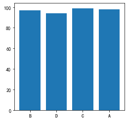
fig, ax = plt.subplots(figsize=(4,4))
_ = ax.boxplot(s.index)
fig, ax = plt.subplots(figsize=(4,4))
_ = ax.hist(np.random.rand(100))
fig, ax = plt.subplots(figsize=(4,4))
_ = ax.pie(data.values, labels=data.index)
练一练
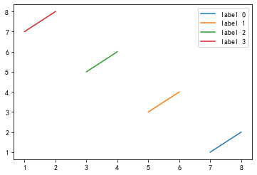
请多次使用plt.plot作图并添加图例标签进行展示。
x = [[1,2],[3,4],[5,6],[7,8]][::-1]
y = [[1,2],[3,4],[5,6],[7,8]]
for i in range(4):
    plt.plot(x[i], y[i], label="label %d"%i)
plt.legend()
<matplotlib.legend.Legend at 0x237aa1fba90>
练一练
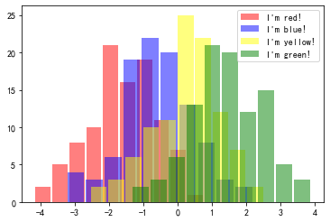
请用手动添加图例的方法来实现plt.hist()例子中自动添加图例的效果。
from matplotlib.patches import Patch
from matplotlib.lines import Line2D
df = pd.concat([
    pd.DataFrame({"num":np.random.randn(100)-1.5, "cat":"A"}),
    pd.DataFrame({"num":np.random.randn(100)-0.5, "cat":"B"}),
    pd.DataFrame({"num":np.random.randn(100)+0.5, "cat":"C"}),
    pd.DataFrame({"num":np.random.randn(100)+1.5, "cat":"D"})
])
c = ["red", "blue", "yellow", "green"]
for i, color in zip(df.cat.unique(), c):
    temp = df.query("cat==@i")
    plt.hist(temp.num, color=color, alpha=0.5, rwidth=0.9)
handles = [
    Patch(edgecolor="None", facecolor="red", alpha=0.5, label="I'm red!"),
    Patch(edgecolor="None", facecolor="blue", alpha=0.5, label="I'm blue!"),
    Patch(edgecolor="None", facecolor="yellow", alpha=0.5, label="I'm yellow!"),
    Patch(edgecolor="None", facecolor="green", alpha=0.5, label="I'm green!")
]
plt.legend(handles=handles)
<matplotlib.legend.Legend at 0x237aa247e20>
练一练
如果把上述代码的plt.axis("off")去除会发生什么?请解释原因。
去除后出现了外层的大边框,这是由于plt当前作用于的是这个最大的1*1子图。
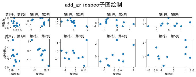
fig, ax = plt.subplots(figsize=(10, 4)) # 只生成1个子图
spec = fig.add_gridspec(nrows=2, ncols=5, width_ratios=[1,2,3,4,5], height_ratios=[1,3])
fig.suptitle('add_gridspec子图绘制', size=20)
for i in range(2):
    for j in range(5):
        ax = fig.add_subplot(spec[i, j]) # 子图分配
        ax.scatter(np.random.randn(10), np.random.randn(10))
        ax.set_title('第%d行,第%d列'%(i+1,j+1))
        if i==1: ax.set_xlabel('横坐标')
        if j==0: ax.set_ylabel('纵坐标')
fig.tight_layout()
练一练
请在心脏病的数据集中选取若干特征按照上述统计量进行定量分析。
略
练一练
请用上述公式,核对pandas中skew()和kurt()的计算结果。
s = pd.Series(np.log(np.random.rand(100)**2))
c = s - s.mean()
n = s.shape[0]
skew = n*n/(n-1)/(n-2)*(c**3).mean()/((c**2).sum()/(n-1))**1.5
skew, s.skew()
(-1.6596070898924549, -1.6596070898924546)
kurt = (n+1)*n*(n-1)/(n-2)/(n-3)*(c**4).sum()/(c**2).sum()**2-3*(n-1)*(n-1)/(n-2)/(n-3)
kurt, s.kurt()
(3.3497831270308462, 3.3497831270308445)
练一练
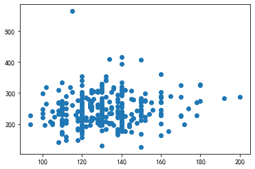
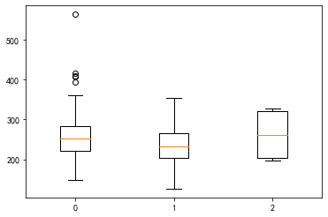
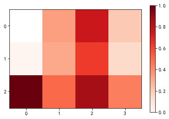
请在心脏病数据集中分别选取数值型-数值型、数值型-类别型、类别型-类别型3种组合的2维变量,利用不同的可视化方法进行观测。
df = pd.read_csv("data/ch11/heart.csv")
plt.scatter(df.trestbps, df.chol)
<matplotlib.collections.PathCollection at 0x237ab5a1d90>
labels = df.restecg.unique()
_ = plt.boxplot([df.loc[df.restecg==i, "chol"].tolist() for i in labels], labels=labels)
res = df.pivot_table(index="slope", columns="thal", values="target", aggfunc="mean")
res.index = res.index.astype("string")
res.columns = res.columns.astype("string")
plt.xticks(range(res.columns.nunique()))
plt.yticks(range(res.index.nunique()))
plt.imshow(res, cmap="Reds")
plt.colorbar()
<matplotlib.colorbar.Colorbar at 0x237ab6e7a00>
练一练
pandas-profiling能够方便地汇总数据信息,但它仍然是不够全面的。请问本文提到的数据观测流程中,哪些环节或方法是pandas-profiling包没有涉及的?
包括但不限于:原生类型和业务类型的精确判断、多个变量关系在同一张图上呈现、针对目标变量的边际分析
一、图片绘制
利用matplotlib完成以下画图问题:
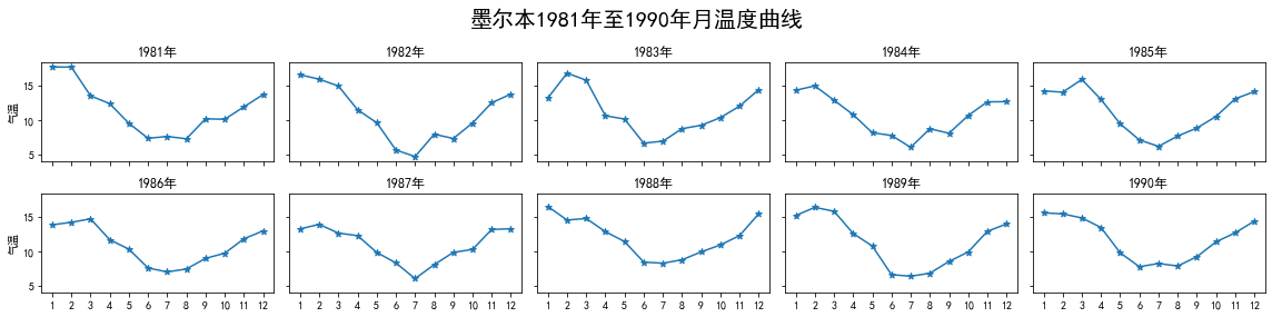
现有1份墨尔本温度的数据集data/ch11/temperature.csv,请仿照图11.38的效果进行绘制。
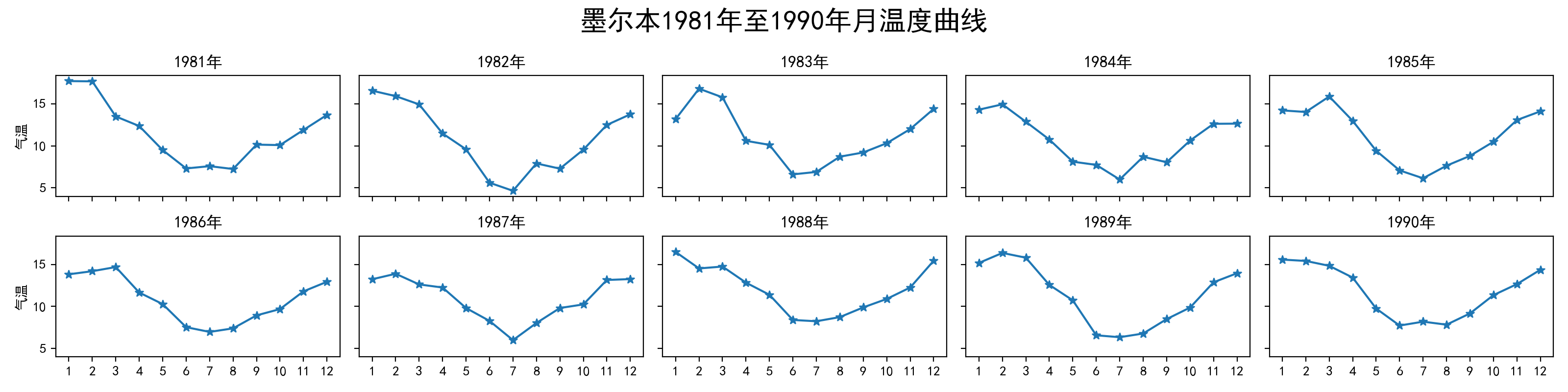
图11.38 墨尔本温度示例图
用np.random.randn(2, 150)生成1组2维数据,做出该数据对应的散点图和边际分布图,效果应如图11.39所示。
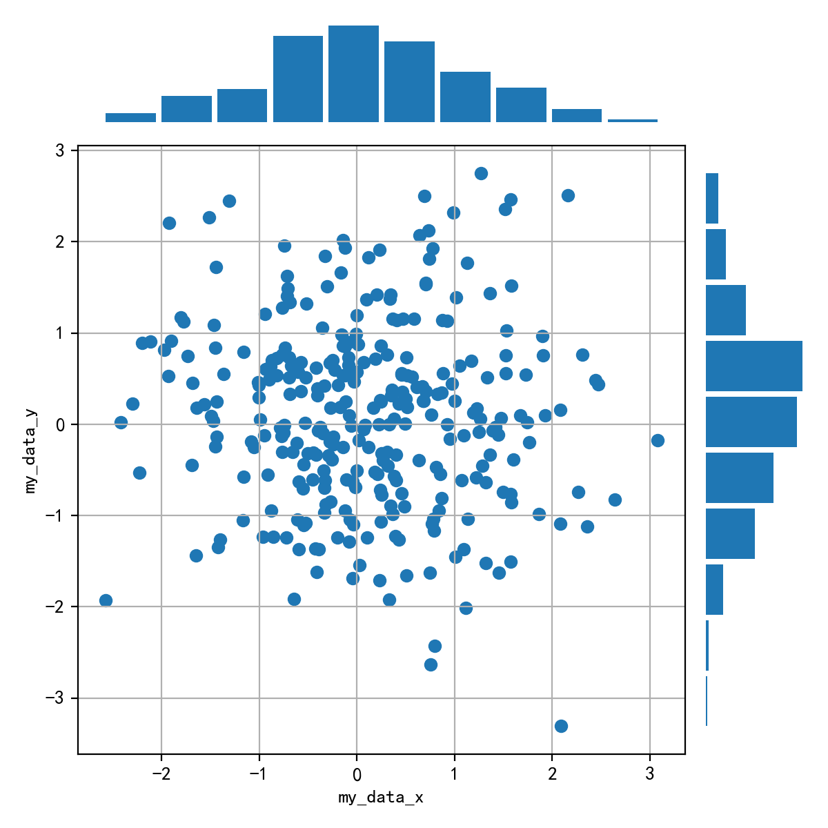
图11.39 正态散点和边际图
提示
图11.39中最上方的边际分布图是指第一行数据的直方图,最左侧的边际分布图是指第二行数据的直方图。
蒙德里安(Piet Cornelies Mondrian)是几何抽象画派的代表人物,图11.40是他某一件作品的局部,请用matplotlib绘制。

图11.40 蒙德里安的某一幅画
某西瓜基地共有10个大棚,工作人员想要对每个大棚的西瓜总产量进行可视化,最终效果如图11.41所示。每个大棚的地理轮廓信息(每行记录为轮廓对应多边形的顶点坐标序列\(x_1,y_1,x_2,x_2,...\))保存在了data/ch11/field.txt中,相应西瓜的生产记录表(包含产地坐标以及当次记录的产量output)保存在了data/ch11/watermelon.csv中。请结合本章知识和给定的数据,模仿图11.41进行绘制。

图11.41 西瓜种植基地中各大棚总产量可视化结果
【解答】
1
fig, axs = plt.subplots(2, 5, figsize=(16, 4),sharey=True, sharex=True)
fig.suptitle('墨尔本1981年至1990年月温度曲线', size=20)
df = pd.read_csv("data/ch11/temperature.csv")
data = df.Temperature.values.reshape(10,12)
time = [[str(j) for j in list(range(1,13))] for i in range(10)]
year = list(range(1981,1991))
for i in range(2):
    for j in range(5):
        axs[i][j].plot(time[5*i+j],data[5*i+j])
        axs[i][j].scatter(time[5*i+j],data[5*i+j],marker='*')
        axs[i][j].set_title(str(year[5*i+j])+'年')
        if j==0: axs[i][j].set_ylabel('气温')
fig.tight_layout()
2
#方法一:利用2*2布局

data = np.random.randn(2, 150)
fig = plt.figure(figsize=(6, 6))
spec = fig.add_gridspec(nrows=2, ncols=2, width_ratios=[6,1], height_ratios=[1,6])
ax = fig.add_subplot(spec[0, 0])
ax.axis('off')
ax.hist(data[0], rwidth=0.9)
ax = fig.add_subplot(spec[1, 0])
ax.scatter(data[0], data[1])
ax.set_ylabel('my_data_y')
ax.set_xlabel('my_data_x')
ax.grid()
ax = fig.add_subplot(spec[1, 1])
ax.hist(data[1], orientation = 'horizontal', rwidth=0.9)
ax.axis('off')
fig.tight_layout()
#方法二:利用7*7布局

fig = plt.figure(figsize=(6, 6))
spec = fig.add_gridspec(nrows=7, ncols=7)
ax = fig.add_subplot(spec[0, :6])
ax.axis('off')
ax.hist(data[0], rwidth=0.9)
ax = fig.add_subplot(spec[1:, :6])
ax.scatter(data[0], data[1])
ax.set_ylabel('my_data_y')
ax.set_xlabel('my_data_x')
ax.grid()
ax = fig.add_subplot(spec[1:, 6])
ax.hist(data[1], orientation = 'horizontal', rwidth=0.9)
ax.axis('off')
fig.tight_layout()
3
from matplotlib.patches import Rectangle
import matplotlib.pyplot as plt
fig, ax = plt.subplots(figsize=(4,4))
patch = Rectangle((0,0),1,1,facecolor='black')
ax.axis("off")
ax.add_patch(patch)
ax.add_patch(Rectangle((0,0.7),0.2,0.3,facecolor='#FFFEEE'))
ax.add_patch(Rectangle((0,0.25),0.2,0.39,facecolor='#FFFEEE'))
ax.add_patch(Rectangle((0.25,0),0.6,0.2,facecolor='#FFFEEE'))
ax.add_patch(Rectangle((0.88,0.13),0.12,0.07,facecolor='#FFFEEE'))
ax.add_patch(Rectangle((0.88,0),0.12,0.09,facecolor='#FFEE58'))
ax.add_patch(Rectangle((0.88,0),0.12,0.09,facecolor='#FFEE58'))
ax.add_patch(Rectangle((0,0),0.20,0.2,facecolor='#3C88D4'))
ax.add_patch(Rectangle((0.25,0.25),0.75,0.75,facecolor='#EE5C5C'))
<matplotlib.patches.Rectangle at 0x237aba9eac0>

4
from matplotlib.path import Path
from matplotlib.collections import PolyCollection
fig, ax = plt.subplots(figsize=(4,4))
with open("data/ch11/field.txt") as f:
    points = [i.split() for i in f.readlines()]
    points = [list(zip(i[0::2], i[1::2])) for i in points]
L = []
for p in points:
    mask = Path(p).contains_points(np.stack([x, y], -1))
    L.append(val[mask].sum())
poly_collections = PolyCollection(
    points,
    array=L,
    cmap="coolwarm",
    edgecolors='black',
)
plt.colorbar(poly_collections, ax=ax)
ax.add_collection(poly_collections)
plt.scatter(x, y, s=val**3/500000, c="black")
ax.set_xlim(-.5,10.5)
ax.set_ylim(-.5,10.5)
ax.set_xticks([])
ax.set_yticks([])
[]

二、数据观测实战
请用本章所学的各种数据观测方法,对如下的2个数据集进行观测分析:
空气污染数据集:data/ch11/pollution.csv
地震记录数据集:data/ch11/earthquake.csv
【解答】
略
三、基于PyOD库的异常检测
异常检测是一种特殊的数据分布度量,它是数据科学领域的重要研究课题之一。PyOD是一个专注于异常检测的Python库,目前已经内置实现了30多种异常检测算法,其项目文档的地址是https://pyod.readthedocs.io/en/latest/,我们可以通过pip安装:
pip install pyod
我们首先使用PyOD的内置数据生成器来生成1组含有异常的数据,如图11.42所示:
from pyod.utils.data import generate_data
# contamination表示异常比例
# behavior设为new表示返回的顺序为先X后y
X_train, X_test, y_train, y_test = generate_data(
    n_train=200, n_test=100, n_features=2,
    contamination=0.1, behaviour="new", random_state=42)
plt.scatter(X_train[:,0], X_train[:,1])

图11.42 模拟生成的含异常样本数据
PyOD的使用非常便利,我们只要导入模型后使用fit()函数进行训练,利用clf.labels_和predict()函数就能分别得到训练集的模型判断结果和测试集的模型判断结果,若为1则异常。此处,我们使用基于KNN的异常检测模型进行演示:
from pyod.models.knn import KNN
clf = KNN()
clf.fit(X_train)
y_train_pred = clf.labels_ # 训练集预测标签
y_test_pred = clf.predict(X_test) # 测试集预测标签
y_test_pred.mean() # 测试集中预测为异常的约有12%
0.12
提示
clf.decision_scores_、clf.decision_function(X_test)和clf.predict_proba(X_test)能够分别得到训练集的样本异常得分、测试集的样本异常得分以及训练集的样本异常概率。
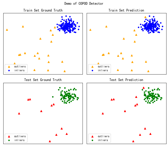
在官网的案例中给出了图11.43中所示的模型结果,它也基于上述的KNN异常检测模型,并且所使用数据集的构造方式与我们完全一致。图11.43的构成如下:左上角为训练集中真实的异常值和非异常值,右上角为训练集中预测的异常值和非异常值,左下角为测试集中真实的异常值和非异常值,右下角为测试集中预测的异常值和非异常值。请利用PyOD中的COPOD模型,仿照图11.43的布局画出类似的实验结果图。
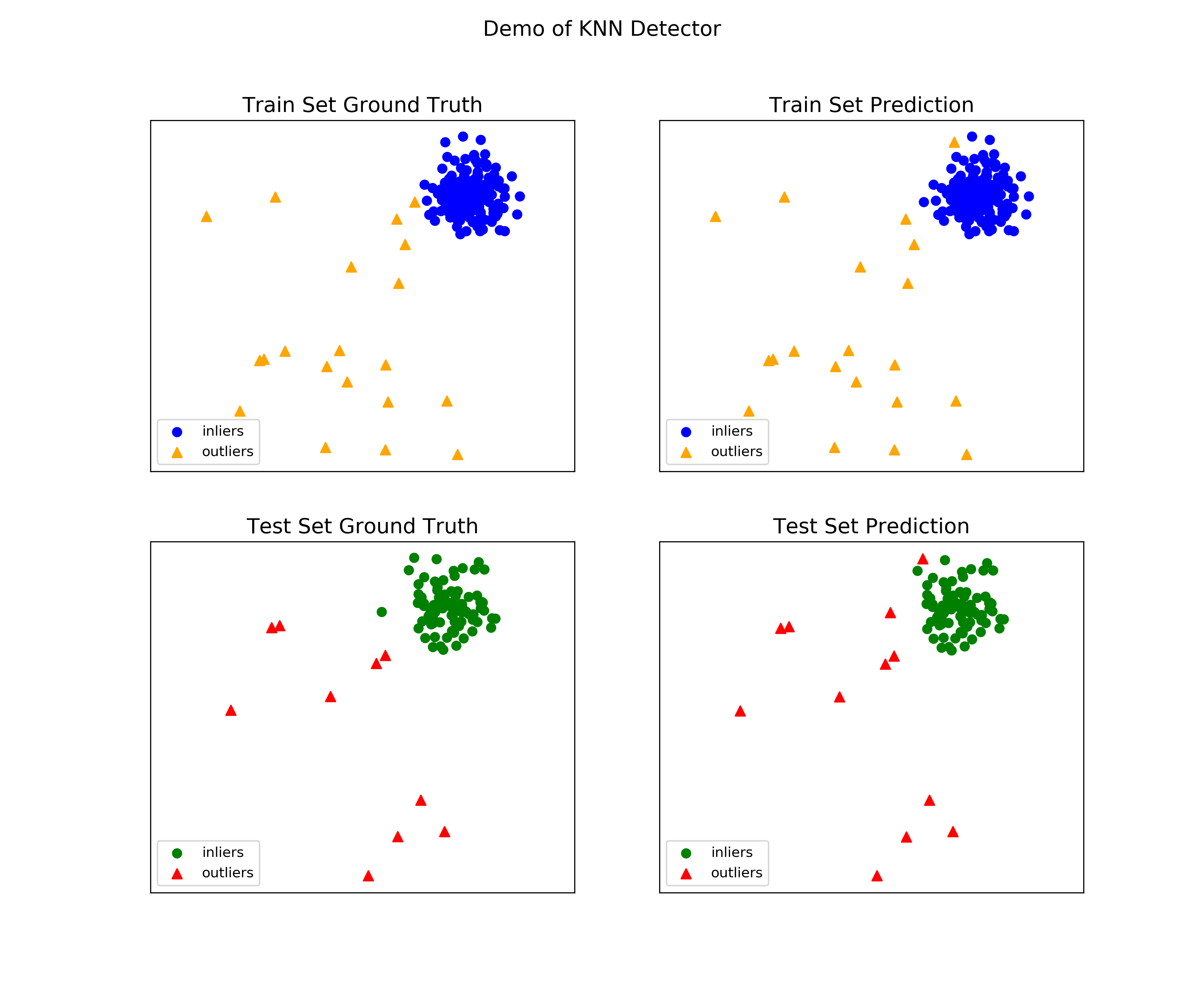
图11.43 基于KNN的检测结果
【解答】
fig, axs = plt.subplots(2, 2, figsize=(8,7), sharex=True, sharey=True)
fig.suptitle('Demo of COPOD Detector')
#00
axs[0][0].scatter(
    X_train[y_train==1, 0], X_train[y_train==1, 1],
    label="outliers", marker="^", c="orange")
axs[0][0].scatter(
    X_train[y_train==0, 0], X_train[y_train==0, 1],
    label="inliers", marker="o", c="blue", s=15)
axs[0][0].set_title("Train Set Ground Truth")
axs[0][0].set_xticks([])
axs[0][0].set_yticks([])
axs[0][0].legend(loc=3)
#01
axs[0][1].scatter(
    X_train[y_train_pred==1, 0], X_train[y_train_pred==1, 1],
    label="outliers", marker="^", c="orange")
axs[0][1].scatter(
    X_train[y_train_pred==0, 0], X_train[y_train_pred==0, 1],
    label="inliers", marker="o", c="blue", s=15)
axs[0][1].set_title("Train Set Prediction")
axs[0][1].set_xticks([])
axs[0][1].set_yticks([])
axs[0][1].legend(loc=3)
#10
axs[1][0].scatter(
    X_test[y_test==1, 0], X_test[y_test==1, 1],
    label="outliers", marker="^", c="red")
axs[1][0].scatter(
    X_test[y_test==0, 0], X_test[y_test==0, 1],
    label="inliers", marker="o", c="green", s=15)
axs[1][0].set_title("Test Set Ground Truth")
axs[1][0].set_xticks([])
axs[1][0].set_yticks([])
axs[1][0].legend(loc=3)
#11
axs[1][1].scatter(
    X_test[y_test_pred==1, 0], X_test[y_test_pred==1, 1],
    label="outliers", marker="^", c="red")
axs[1][1].scatter(
    X_test[y_test_pred==0, 0], X_test[y_test_pred==0, 1],
    label="inliers", marker="o", c="green", s=15)
axs[1][1].set_title("Test Set Prediction")
axs[1][1].set_xticks([])
axs[1][1].set_yticks([])
axs[1][1].legend(loc=3)
fig.tight_layout() # 调整子图的相对大小使字符不会重叠